Prev: Binary Heaps Part 1
- by Brad Bart, Simon Fraser University
- Elementary Data Structures
- Linked Structures 1: Binary Search Trees
- Linked Structures 2: Binary Heaps Part 1
- Linked Structures 2: Binary Heaps Part 2
Running Time Mirage
You left Part 1, yesterday1, with a simple implementation for a priority queue: an unsorted array. Although the cost to insert was a delightful O(1), the cost to remove the min was an unfriendly O(n).
Augmenting the array with an index for fast reference to the min was a sharp idea. The index makes a linear search for the min unnecessary and it is maintainable in O(1) on insert. That's all good, except for one catch.
The index is not maintainable in O(1) on remove.
Why? Although it is O(1) to find the min and remove it, once it is gone, what's the index of the next min? Locating it will require a linear search resulting in O(n) steps, which means you are no better off than you were without the augmentation.
Another Recursive Definition
To index the min was still a sharp idea, however. The strategy would have worked if only it was easy to find the next min, like as easy as a single comparison.
Perhaps it would be possible to apply Divide & Conquer if you organized the elements as follows:

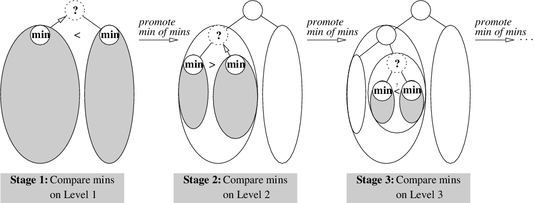
As before, the min (at the top) is easy to locate and remove. The rest of the elements are divided up into two roughly equally sized pools, which will, if defined recursively, also have mins that are easy to locate and remove. So, when you remove the min and need to find the next min, it must be the smallest of the min of the left pool and the min of the right pool.
As with the last augmentation, you might prematurely conclude that the running time for remove is now back down to O(1). Unfortunately, it's going to require more effort than just 1 simple comparison. Here's why.
1 If it wasn't yesterday, then return HTTP
status code 412. Please press the back
button in your browser and try again tomorrow.
When you remove the min, it leaves a hole. And, you find the
next min by finding the min of mins, and promote it
to where the hole was. The problem is that promoting the new
min leaves a hole in one of the pools, which will, by induction,
have to be filled as well. That means another comparison, another
promotion, another hole to fill, and so on.
Therefore the running time is not going to be as fantabulous
as O(1).
But because each successive comparison works on pools that are
roughly
half
the size, the running time will
clock in at an excellent O(log n).
Once again, a recursive definition leads to an excellent
implementation that is reminiscent of a binary tree.
Note that maintaining the balance between the two pools
is a tricky detail. It's possible to do it in several
ways, but no matter which way you choose, the running time
for insert will rise to O(log n).2
2 Yes, keener. A Fibonacci heap has
O(1) insert. But it doesn't really stick to
two pools, either.
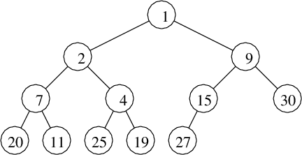
Example of a Binary Heap:
Binary Heap: Array Representation
Binary Heap
So, define a binary heap to be a balanced binary tree
whose keys are arranged as described above.
Stated formally:
Implementation
To implement insert and remove, do what is colloquially
called
“trickle-up” or
“trickle-down”:
a sequence of node swaps to mend the heap property when
a node is inserted or removed.
Algorithm for Trickle-Up: If smaller than parent, then swap and recurse
Algorithm for Trickle-Down: If larger than either child, then swap with the smallest child and recurse
Running Times
The running time of insert equals the running time of trickle-up,
because all of the other operations are O(1). Since:
The same analysis holds for remove and trickle-down, and so
all operations run in an excellent
O(log n).
Summary
Armed once again with wishful thinking, you stated
the desired properties using a recursive
definition, and this time you were rewarded with a binary heap.
In comparison to the binary search tree where the invariant was
left ≤ x < right, the binary heap had the invariant
x ≤ left, right.
This made it easy to find the min because, by mathematical induction,
the root must be the min.
But finding the min and removing the min are two different problems.
Fortunately, this invariant also made it easy to find the second min:
it must be one of the two children of the root.
This was yet another example of how Divide & Conquer can
lead to an excellent O(log n) running time.
Conclusion
And that's probably a good place to wrap this up.
You look like you could use a recap:
You started with a review of induction from your roots in proving
math results, both vanilla inductions and strong inductions.
Next, you applied these techniques to prove some results about
the behaviour of algorithms.
It turned out that the easiest algorithms on which to use induction were
recursive, and you concluded that
“induction” and “recursion”
are essentially the same word.
Finally, you applied induction to
some recursive designs, the binary search tree and the binary heap,
which are two of the data structures you will learn in CMPT 225.
You have now completed the workshop on Mathematical Induction!
Perhaps you've seen some of this before; perhaps most of it was
new to you. But either way, hopefully you feel enriched, titilated
and entertained1 . . .
. . . or at least amply prepared for what you, a CMPT 225
student, should know about Mathematical Induction before taking CMPT 225.
1Yes, the good kinds of math contain much creativity,
and tend to evoke these kinds of feelings.


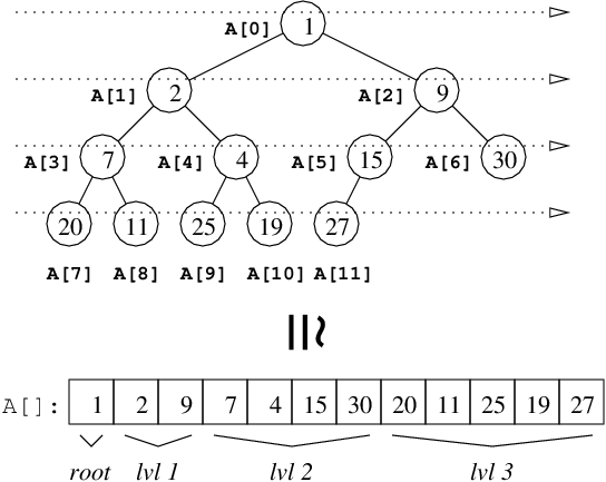
That the tree is complete is not only a very clean way to
impose balance on the tree, it also means that the nodes can
be conveniently stored in a contiguous array
A[0..n-1] that
follows its level-order traversal. [figure left] Hopefully,
you can spot a pattern among the indices that would make it
easy to locate the left child, right child and parent.
(Don't worry - I won't make you prove this by induction.)
void insert(int key, int priority) {
  A[len++] = Node(key, priority);

  // the new node might have priority smaller
  // than its ancestors, so . . .
  trickleup(len-1);
}

int remove() {
  int ret = A[0].key;

  A[0] = A[--len];

  // the new root might have priority larger
  // than its ancestors, so . . .
  trickledown(0);

  return ret;
}

therefore, the running time of
trickle-up is
O(h) = O(log2n).
