Prev: Loop Invariants

What Every CMPT 225 Student Should Know About Mathematical Induction

- by Brad Bart, Simon Fraser University

Part 1: Overview of Induction

• Summary
• The Inductive Step
• The Basis Cases

Part 2: How Induction Relates to Computer Science

• Programming Using Induction
• Loop Invariants
• Invariants and Recursive Algorithms

Part 3: Induction in CMPT 225

• Elementary Data Structures
• Linked Structures 1: Binary Search Trees
• Linked Structures 2: Binary Heaps

Part 2: How Induction Relates to Computer Science

Invariants and Recursive Algorithms

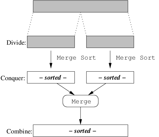
Recursive Algorithms often solve problems by the Divide & Conquer paradigm, which involves three stages:
divide, conquer and combine.

• Divide the problem into 2 or more smaller subproblems, whose solutions are strongly related to the solution of the original problem.

• Conquer by calling the recursive algorithm on each subproblem.

• Combine together the subproblem solutions to form the solution to the original problem.

As an example of Divide & Conquer, consider Merge Sort. In this sorting algorithm, the list is divided into two “equal” parts, i.e., within size 1 of each other. Next, each part is sorted recursively, the conquer stage. Finally, the two sorted sublists are combined in a Merge operation, which iteratively compares and transfers the min of the two lists. The recursion stops when Merge Sort is called on an array of size 1, which is trivially sorted.¹

¹It might be better to terminate the recursion at, say, any array of size n < 15, because an alternate sorting algorithm, like Insertion Sort, will perform better than Merge Sort for small n.

// sorts A[first..last]
void msort(int *A, int first, int last) {
  // base case
  if (first >= last) return;

  // divide
  int mid = (first+last) / 2;

  // conquer
  msort(A, first, mid);
  msort(A, mid+1, last);

  // combine
  merge(A, first, mid, last);
}

Just like an inductive step for a strong induction, you may assume that the algorithm is correct for all smaller cases, and therefore the conquer stage correctly sorts the two sublists A[first..mid] and A[mid+1..last]. Since the merge(...) step results in a sorted A[first..last], the algorithm is correct.

This expeditious analysis illustrates how powerful invariants are for proving the correctness of recursive algorithms.

The analysis of the running time is similar. Let T(n) represent the number of steps to Merge Sort an n element array. When n ≤ 1, the array A is trivially sorted (base case), and the running time is O(1). When n > 1, a certain number of steps are taken for each of the Divide, Conquer and Combine stages.

• Divide: To compute the value of mid costs O(1) time.

• Conquer: The lower half of the array has ⎡n/2⎤ elements and the upper half has ⎣n/2⎦. To recursively sort them will cost T(⎡n/2⎤) + T(⎣n/2⎦) steps.

• Combine: What is the time required to merge n elements? At each step, the smallest un-merged element of the lower half is compared with the the smallest un-merged element of the upper half. The smaller of the two is the minimum of all un-merged elements, and is placed in its correct position. Since each element is placed exactly once, the number of steps is linear, i.e., O(n).

Therefore, the recursive definition of T(n) is:

T(n) =	{	O(1)  if n ≤ 1
		O(1) + T(⎡n/2⎤) + T(⎣n/2⎦) + O(n)  if n > 1

The next step is a familiar one: guess an expression for T(n) and then use induction to prove it is correct. Because you remember past discussions of the running times of sorting algorithms, you guess that T(n) = O(n log n), i.e., for constants c, n₀, the inequality T(n) ≤ c⋅n log n holds for every n ≥ n₀.

The algebra involved in the inductive step is beyond the scope of CMPT 225: you will do proofs like this when you take CMPT 307. If you just can't wait until then, click here.

You will write and prove your own loop invariants in CMPT 225: some will be about the algorithm's progress/correctness; some about its running time. Induction has another use however— as applied to the development and analysis of data structures. This is the subject of Part 3.