Prev: Invariants and Recursive Algorithms

What Every CMPT 225 Student Should Know About Mathematical Induction

- by Brad Bart, Simon Fraser University

Part 1: Overview of Induction

• Summary
• The Inductive Step
• The Basis Cases

Part 2: How Induction Relates to Computer Science

• Programming Using Induction
• Loop Invariants
• Invariants and Recursive Algorithms

Part 3: Induction in CMPT 225

• Elementary Data Structures
• Linked Structures 1: Binary Search Trees
• Linked Structures 2: Binary Heaps

Part 3: Mathematical Induction in CMPT 225

So far, you discovered that mathematical induction is not merely good for verifying sums, drinking 99 bottles of beer, or driving across Saskatchewan!¹ You can apply mathematical induction and its partner, recursion, to prove the correctness and the running time of algorithms.

¹For those who haven't taken the drive, the Saskatchewan landscape approximates a sequence of equally spaced grain fields, as seemingly endless as a ladder with an infinite number of rungs.

Mathematical induction is also the central theme in the development and analysis of data structures with efficient implementations.

Elementary Data Structures

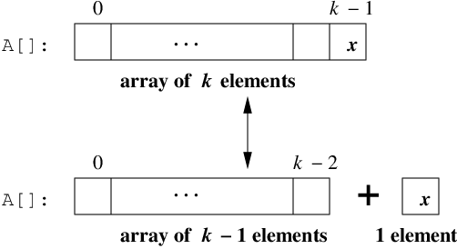
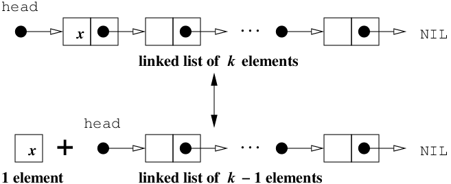
In your intro computing class[es], they probably told you that the universe was composed of exactly two data structures: the array and the linked list. What they probably didn't tell you was that both arrays and linked lists are recursive in that you can build a larger one by adding an element to an incrementally smaller one.

Recursive Definition of an Array:

Recursive Definition of a Linked List:

This means that you can prove the correctness and the running time of algorithms on these data structures by using simple induction, much like you did for Insertion Sort.

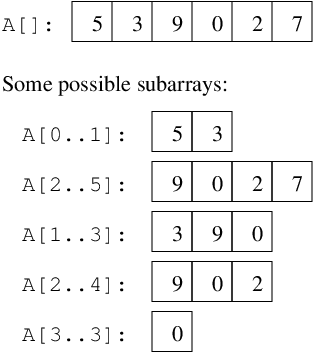
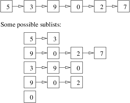
Similarly, within an array you can find many smaller subarrays, and not just the incrementally smaller ones. The same can be said for the sublists of a linked list.

There are many subarrays within each array:

        

There are many sublists within each linked list:

        

This means you can prove the correctness and the running time of algorithms on these data structures by using strong induction, much like you did for Merge Sort. The subarrays for Merge Sort were two equally sized pieces, but in general, Divide & Conquer doesn't restrict the numbers or the sizes of the subarrays. It's possible to divide into 3 or 4 equally sized pieces, or perhaps two pieces with a ⅓ − ⅔ split.

Case Study: Dynamic Set Implementation Using an Array

A dynamic set is a data container that provides two operations, insert [a key] and search [for a key]. (Other operations are also possible, but these two will be enough to make the problem interesting.)

Thus, a dynamic set's operations are very much like those of a database: you insert information to be retained and retrieved at a later stage. What you should choose as a collection of keys is a matter of convenience. For example, you would usually look up a person in the phonebook white pages (or your cell phone's contacts list), by using their name, but usually not by their phone number or street address. One way is convenient, the other way is . . . not.

And as the size of the dynamic set increases to the millions, or perhaps billions, you want the operations to be as convenient as possible.

For the purpose of the discussion, let n represent the current size of the dynamic set, i.e., the number of keys it currently holds. In the implementation, the array A[] will be indexed from 0, and the variable len will maintain n, the current number of keys.

 

 

Some of you keen math types might be asking yourselves: How many different [nonempty] subarrays of an n-element array are there? The quick answer is: a lot. Perhaps a more precise answer is n(n + 1)/2.

Another good one: How many ways can you chop up an n element array into two or more subarrays? Again, it's a lot: 2ⁿ⁻¹ − 1.

The neat thing is that both questions can be answered using the math you learned from MACM 101.

To build a dynamic set using a data structure, you have to think about how to lay out the data within your structure. In this case study, the data are the n keys and the data structure is the array.

There are two “obvious” approaches:

1. Store the keys in the first n slots of the array,
   in any order.

2. Store the keys in the first n slots of the array,
   in sorted order.

At this point, you should take a few moments to think about how you would implement insert and search using each approach: four functions in all. Also consider the running time of each operation.

Once you have formed your answers, proceed to the implementation in the next part.