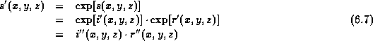
An image can be expressed as the product of illumination and reflectance:

Now define:
Then:

or:

where  is the Fourier transform of
  and
and
 is the Fourier transform of
  .
.
We then apply a filter to  :
:
In the spatial domain:
We then exponentiate  to get the enhanced image:
Now  and
and  are the illumination and
reflectance of the ``enhanced'' image. The illumination component
tends to vary slowly across the image. The reflectance tends to vary
rapidly. Therefore, by applying a frequency domain filter such as that
in Figure 6.1, we can reduce intensity variation across the
image while highlighting detail. This approach is summarized in
Figure 6.2.
are the illumination and
reflectance of the ``enhanced'' image. The illumination component
tends to vary slowly across the image. The reflectance tends to vary
rapidly. Therefore, by applying a frequency domain filter such as that
in Figure 6.1, we can reduce intensity variation across the
image while highlighting detail. This approach is summarized in
Figure 6.2.
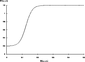
Figure 6.1: Cross section of a spherically symmetric
homomorphic filter.  is the distance from the origin.

Figure 6.2: Homomorphic Filtering Block Diagram
Although homomorphic filtering in the spectral domain is conceptually
simple, its implementation becomes unwieldy when dealing with large
images. The 3D volume of MR data is very large when transformed to complex
floating point values by the DFT; the size of Data Set 1 is  (
( ). The filter itself is the same size as the
data volume. The result of this vast amount of data is considerable
memory page swapping. Thus execution can be quite slow.
). The filter itself is the same size as the
data volume. The result of this vast amount of data is considerable
memory page swapping. Thus execution can be quite slow.
The second problem encountered with spectral domain homomorphic
filtering is circular convolution. Multiplication in the spectral
domain is equivalent to convolution in the spatial domain. The result
of the convolution of the MR image with the spatial kernel,
 , corresponding to the spectral domain filter,
 , (see Equation 6.8) is an image that is
larger than the original by the size of the spatial mask. The excess
data are wrapped and added to the opposite sides of the image in the
spatial domain if not accounted for in the spectral domain.
, (see Equation 6.8) is an image that is
larger than the original by the size of the spatial mask. The excess
data are wrapped and added to the opposite sides of the image in the
spatial domain if not accounted for in the spectral domain.
This wrapping, illustrated in one dimension in Figure 6.3 (see Numerical Recipes in C, p.541 [42]), is a property of spectral domain filtering. It can be avoided by padding the original image with zeros at its boundaries to compensate for the mask size, then discarding the padded region after filtering. Although this solution sounds simple, it increases the size of the image to be processed and results in undesirable FFT sizes.
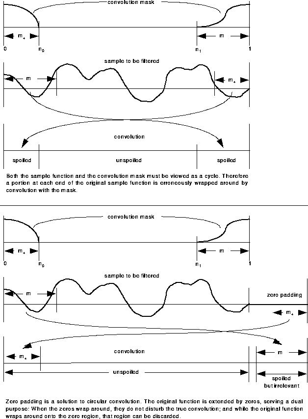
Figure 6.3: Circular Convolution