18. Polar Coordinates

In these notes you will learn:

• How to convert between polar and Cartesian coordinates

18.1. Introduction

Sometimes it can be useful to convert from Processing’s coordinate system to a polar coordinate system. This is particularly useful when we want to make objects move in a circle.

18.2. Cartesian Coordinates

Processing uses a Cartesian coordinate system where the coordinates of a point (or a pixel) are given by the horizontal and vertical distance from the origin. As we’ve learned, the origin for the image window in Processing is the top left hand corner (although it can be moved by using the translate function).

18.3. Polar Coordinates

We can represent a point by using polar coordinates. In the polar coordinate system a point is represented by how far away from the origin it is, and its angle from the origin. The angle is usually referred to as theta.

18.4. Coordinate Conversion

Processing has functions that make it simple to convert between Cartesian and Polar coordinates.

To translate from polar coordinates to Cartesian coordinates, where the Cartesian coordinates are specified by the variables x and y, and the polar coordinates by the variables r (the distance from the origin) and theta:

x = r * cos(theta);
y = r * sin(theta);

And to translate from Cartesian coordinates to polar coordinates:

theta = atan2(y,x); //theta in radians
r = sqrt(sq(x) + sq(y));

These formulae assume that the origin is the top left hand corner of the window. If we wanted the origin to be somewhere else (like the centre of the window) we would have to add or subtract amounts from the x and y coordinates as appropriate, or use the translate function to move the origin.

Assume that we want to find the polar coordinates of a point, using the centre of 200x200 window as the origin. We would have to use x and y values that are relative to the centre of the window. If x = 40 and y = 150 the polar coordinates would be:

theta = atan2((150 - 100), (40 - 100)); //= 2.44 radians
r = sqrt(sq(-60) + sq(50)); //= 78.1

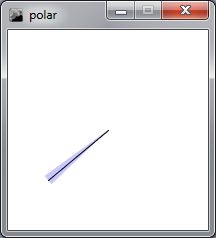
This Processing program draws an arc and a line from the centre of the window to the point {40, 150}. The program uses the polar coordinate conversion formulae to calculate the angle and radius of the arc:

float theta;
float r;
float x;
float y;

void setup(){
  size(200, 200);
  background(255);
  smooth();

  x = 40;
  y = 150;

  theta = atan2((y - height/2), (x - width/2));
  r = sqrt(sq(x - width/2) + sq(y - height/2));
  println(theta);
  println(r);
  noStroke();
  fill(200,200,255);
  arc(width/2, height/2, r*2, r*2, theta-PI/45, theta+PI/45);

  stroke(1);
  line(width/2, height/2, x, y);

  println( atan2((y - 250), (x - 250)) );
  println( sqrt(sq(x - 250) + sq(y - 250)) );
}

The output of this program looks like this:

Recall that the arc function takes six parameters:

arc(x, y, width, height, start, stop)

In the program shown above I’ve used polar distance as the radius of the arc and centred the arc on the angle theta. The line drawn from the centre of the window to x, y = {40, 150} appears down the centre of the arc.

18.5. Circle of Circles

Here is a small Processing program that draws a circle (of circles) around the centre of the window. A circle is to be drawn every 12 degrees:

float theta;
float r;
float x;
float y;
float grey;

void setup(){
  size(500, 500);
  smooth();

  theta = 0;
  r = 150;

  // Draw 30 circles around centre
  for(theta = 0; theta < TWO_PI; theta += TWO_PI/30){
    x = r * cos(theta) + 250;
    y = r * sin(theta) + 250;
    grey = map(theta, 0, TWO_PI, 0, 255);
    fill(grey);
    ellipse(x, y, 10, 10);
  }
}

The output of this program looks like this:

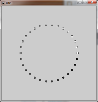
I’ve drawn each circle in a different shade of grey, if I changed the color mode to HSB and used the grey value for the hue I would get a different (and more colourful) image.