18. Sorting and Searching a vector
Now we come to sorting, which is an important and well-studied topic in computer science. Sorting a vector means to arrange its elements in order from smallest to largest.
Hundreds of different sorting algorithms have been created. Here we will only look at one of the most efficient simple sorting methods known as insertion sort.
We will restrict our attention to sorting vector<int> objects for simplicity, and also assume there are duplicate numbers among the values being sorted.
18.1. Linear Insertion Sort
Linear insertion sort is a simple (but slow!) sorting algorithm that you are probably already familiar with: many people use it to sort their cards when playing card games. For brevity, we usually refer to it as just insertion sort.
Here’s the idea. Suppose we want to arrange these values into ascending order:
5 6 1 2 4
Insertion sort conceptually divides this lists into a sorted part and an unsorted part:
sorted    unsorted
     5 |  6  1  2  4
The | is an imaginary line that shows where the sorted/unsorted portions begin/end. Initially, only the first element is on the sorted part, and the rest are on the unsorted part.
Insertion sort now repeats the following until the unsorted part is empty:
- Take the first element of unsorted and insert it into its correct position in sorted (so that sorted is always in ascending sorted order).
Lets trace this on our sample data:
5  |  6  1  2  4

5  6  |  1  2  4

1  5  6  |  2  4

1  2  5  6  |  4

1  2  4  5  6  |
Note that finding the insertion point requires some searching. Typically, we use a variation of linear search to do this, hence the name linear insertion sort. It’s also possible to do the insertion using binary search (discussed below). In that case, the algorithm is called binary insertion sort.
How fast is insertion sort? Not very, it turns out. To estimate it’s performance, note that n - 1 insertions are needed to sort an n-element vector. Each insertion requires doing a linear search followed by an insertion. We can’t get an exact count of how many comparisons (the standard measure of sort efficiency) insert sort does without knowing the details of the data being sorted, but we can make a useful worst-case estimate.
So for the sake of simplifying the analysis, suppose that the linear search part of insertion sort always does the worst-case number of comparisons, i.e. it always searches to the end of the sorted part of the list. Then suppose we are sorting 5 numbers:
a | b c d e     0 comparisons to determine location of a
a b | c d e     1 comparison to determine location of b
a b c | d e     2 comparisons to determine location of c
a b c d | e     3 comparisons to determine location of d
a b c d e |     4 comparisons to determine location of e
This shows that, in the worst case,  comparisons
are needed to sort 5 objects. Generalizing this is not too hard: to sort n
objects, then, in the worst case,
comparisons
are needed to sort 5 objects. Generalizing this is not too hard: to sort n
objects, then, in the worst case, 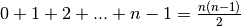 comparisons will be done. The expression
 is quadratic, because the power of its highest term
is 2. This tells us that as n gets bigger, the number of comparisons done by
insertion sort grows like
is quadratic, because the power of its highest term
is 2. This tells us that as n gets bigger, the number of comparisons done by
insertion sort grows like  .
.
This analysis only considers comparisons: it ignores the work done when
inserting new elements. So lets consider how many numbers are moved by
insertion sort. In the worst case, insertion sort does the most work when we
insert a number at the beginning of the vector (because it has to move all
the elements after it up 1 position). In a vector with  elements,
inserting an item at the beginning requires moving
elements,
inserting an item at the beginning requires moving  elements.
Since, in the worst case, we will be inserting elements at the
start (not — the first element is always automatically considered
to be sorted),
elements.
Since, in the worst case, we will be inserting elements at the
start (not — the first element is always automatically considered
to be sorted),  items must be
moved.
items must be
moved.
So whether you count comparisons or data moves, the result is the same. To
sort n items in a vector, linear insertion sort takes time proportional to
. In practice, this turns out to be quite slow, and insertion sort
is really only useful for sorting a small number of items (maybe a few
thousand, depending upon the speed of your computer).
Here’s an implementation of insertion sort:
void insertion_sort(vector<int> v) {
  for(int i = 1; i < v.size(); ++i) {

    int key = v[i];             // key is the value we are going to insert
                                // into the sorted part of v

    int j = i - 1;              // j points to one position before the
                                // (possible) insertion point of the key;
                                // thus, key will eventually be inserted at
                                // v[j + 1]

    //
    // This loop determines where to insert the key into the sorted part
    // of v. It does this by searching backwards through the sorted part of v
    // for the first value that is less than, or equal to, key.
    //
    // This loop combines searching with element moving. Every time an element
    // bigger than the key is found, it is moved up one position.
    //
    // It's possible that there is no value in the sorted part that is
    // smaller than key, in which case key gets inserted at the very
    // start of v. This is a special case that is handled by the j >= 0 term
    // in the loop condition.
    //
    while (j >= 0 && v[j] > key) {
      v[j + 1] = v[j];
      --j;
    }
    // True after loop ends: (j < 0 || v[j] <= key)

    v[j + 1] = key;             // j points to the location *before*
                                // the one where key will be inserted
  }
}
While insertion sort is conceptually simple, you need to be quite careful to get the details exactly right when you implement it. This can be tricky, and so you should test it carefully on a variety of different arrays.
Note
What sorts of arrays should you test insertion sort on? Testing with small arrays is often a good way to find bugs, so we suggest at least the following:
- The empty array, {}.
- An array with one element, e.g. {5}.
- An array with two elements already in sorted order, e.g. {5, 8}.
- An array with two elements not in sorted order, e.g. {8, 5}.
- An array with three elements in sorted order, e.g. {5, 8, 9}.
- An array with three elements in reverse sorted order, e.g. {9, 8, 5}.
- An array with three elements in no particular order, e.g. {5, 9, 8}.
- A larger array, e.g. {7, 5, 3, 9, 0, 8, 1, 5}.
18.2. Faster Sorting
Linear insertion sort is far from being the most efficient sorting algorithm
in practice. For large amounts of data, it runs extremely slowly. More
efficient sorting algorithms exist that perform a number of comparisons
proportional to  . For example, mergesort, quicksort, and
heapsort are three well-know sorting algorithms that all do about
. For example, mergesort, quicksort, and
heapsort are three well-know sorting algorithms that all do about  on average. They are a little more complex than simple sorts like
insertion sort, but they sort large amounts of data much more quickly.
on average. They are a little more complex than simple sorts like
insertion sort, but they sort large amounts of data much more quickly.
Real-world sorting algorithms can be quite complex. For example, timsort is a popular sorting algorithm that
can often do less than comparisons when sorting many real-
world data sets. It does this by identifying parts of the data that are
already partially sorted. Timsort is a very complex algorithm (see the source
code)
consisting of hundreds of lines of carefully crafted C code.
18.3. Binary Search
Sorted data is extremely valuable. One of the best demonstrations of this is the incredible performance of binary search, an algorithm that finds the location of a given element in a sorted vector:
// Pre: v is sorted
// Post: returns an index i such that v[i] == x
int binary_search(int x, const vector<int>& v)
The pre-condition is essential here: binary search only works on data that is in (ascending) sorted order.
Binary search works by repeatedly halving the set of possible elements that might be equal to x. At the start, all elements of v are potentially equal to x, but each comparison cuts the candidate set in half.
For example, suppose our vector looks like this:
4, 5, 8, 11, 15, 20, 21
Does it contain 6? Binary search would do the following:
4, 5, 8, 11, 15, 20, 21
          ^
          |
      check the middle-most element
Since 11 is not 6, we know that if 6 is in the vector, it must be to the left of 11. Thus we can ignore all the elements from 11 to 21:
4, 5, 8
   ^
   |
 check the middle-most element
Since 5 is not 11, we know that if 6 is among these numbers it must be to the right of 5. Thus we can ignore 4 and 5:
8
^
|
check the middle-most element
After checking that 8 is not equal to 6, we are done: we’ve proven that 6 is not in the list of numbers. And it only tool 3 comparisons to do this. In contrast, linear search would have had to have checked all the numbers to make none are 3, and so would have done 7 comparisons.
Here’s an implementation:
// Pre: v[begin] to v[end - 1] is in ascending sorted order
// Post: returns an index i such that v[i] == x and begin <= i < end;
//       if x is not in the range, -1 is returned
int binary_search(int x, const vector<int>& v, int begin, int end) {
  while (begin < end) {
    int mid = (begin + end) / 2;
    if (v[mid] == x) {          // found it!
      return mid;
    } else if (x < v[mid]) {
      end = mid;
    } else if (x > v[mid]) {
      begin = mid + 1;
    }
  }
  return -1;                    // x not found
}

// Pre: v is in ascending sorted order
// Post: returns an index i such that v[i] == x; if x is not in
//       v, -1 is returned
int binary_search(int x, const vector<int>& v) {
  return binary_search(x, v, 0, v.size());
}
The algorithm is rather subtle at points, and so it can be tricky to get it right the first few times you implement it. For example, this line is easy to get wrong:
int mid = (begin + end) / 2;
This calculates the mid-point of a range. You can derive this as follows. The
length of the range is  , and half of that is
 . Since the range starts at
  , the
mid-point is
, the
mid-point is 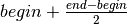 , which simplifies to
 .
.
If happens to be odd, then
ends with .5, and we simply chop that off (e.g. 34.5 becomes 34). This is not
obviously the right thing to do, but if you test it with a few actual values
by hand, and write some good tests, you can be pretty confident that it’s
correct.
Thorough testing is essential for an algorithm like binary search. Here are some sample tests:
void binary_search_test() {
  cout << "binary_search_test called ...\n";
  vector<int> v;                // {}

  assert(binary_search(5, v) == -1);

  v.push_back(6);               // {6}
  assert(binary_search(5, v) == -1);
  assert(binary_search(6, v) == 0);
  assert(binary_search(7, v) == -1);

  v.push_back(10);              // {6, 10}
  assert(binary_search(5, v) == -1);
  assert(binary_search(6, v) == 0);
  assert(binary_search(7, v) == -1);
  assert(binary_search(10, v) == 1);
  assert(binary_search(11, v) == -1);

  cout << "... all binary_search_test tests passed\n";
}
How fast is binary search? Blazingly fast, as it turns out. Every time binary search iterates through its main loop one time, it discards half of all the elements of v. So if v initially has n elements, the number of possible elements that could be equal to x decreases in size like this:
n

n/2

n/4

n/8

n/16

...

n/2^i
Eventually,  is bigger than n, meaning there are no more elements
to consider. We want to know the first value of
is bigger than n, meaning there are no more elements
to consider. We want to know the first value of  that makes
 . That is, we want to solve for in this
inequality:
. That is, we want to solve for in this
inequality:
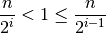
Multiplying everything by gives this:

And taking the base-2 logarithm:
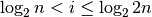
Since  This further
simplifies to:
This further
simplifies to:

Thus, i is approximately equal to  .
.
This result shows that binary search does about  comparisons
in the worst case. Sometimes it might do fewer, of course, but
comparisons
in the worst case. Sometimes it might do fewer, of course, but  is small for even big values of n. For instance,
  , meaning that binary search does at most 30 comparisons to find a given
number in a vector with a billion elements.
, meaning that binary search does at most 30 comparisons to find a given
number in a vector with a billion elements.
Note
One way to think about the base-2 logarithm of a number is
this: is the number of bits used in the binary
representation of n.
Binary search is extremely efficient for searching large amounts of data. But you pay a price: the data must be in sorted order. The problem with sorting is that even the fastest sorting algorithms are slower than linear search. Thus sorting data and then calling binary search is usually slower than doing linear search. However, you only need to sort the data once, and so if you need to do a lot of searches, and sorting the data once followed by many binary searches may be faster than lots of linear searches.
Note
Did you know that you can drive your car a mile without using a drop of gas? Just start at the top of a mile-long hill and roll down. Of course, the hard part is getting your car up there in the first place!
Binary search suffers from a similar problem.