Let's look a little more closely at some of the things these tree structures an do for us.

Binary Search Trees

Lets look at trees that are (1) binary and (2) ordered.
We will use these trees to store some values (in a computer's memory, I assume).
- Each vertex will contain one of whatever data we're storing.
- I'm assuming we're organizing our data by one value: its key.
- The keys must be totally-ordered.
- Let's assume all the keys are distinct for simplicity.
- The key might be something like a student number or name: the thing we want to search by.

That is, it will look like this:

typedef struct bst_node {
    struct bst_node *leftchild;
    struct bst_node *rightchild;
    char *key;
    char *otherdata;
} bst_node;

We'll make a few rules about how we arrange the values in the tree:
- The keys in the left subtree must be less than the key of the root.
- The keys in the right subtree must be greater than the key of the root.
- Those must also be true for each subtree.
A tree like this is called a binary search tree or BST.
For example, this is a binary search tree containing some words (ordered by dictionary ordering):
This is another BST containing the same values:
- We haven't made any assertions about the BST being balanced or full.

It is fairly straightforward to insert a new value into a BST and maintain the rules of the tree.

The idea: look at the keys to decide if we go to the left or right.
If the child spot is free, put it there.
If not, recurse down the tree.

procedure bst_insert(bst_root, newnode)
    if newnode.key < bst_root.key  // insert on the left
        if bst_root.leftchild = null
            bst_root.leftchild = newnode
        else
            bst_insert(bst_root.leftchild, newnode)
    else  // insert on the right
        if bst_root.rightchild = null
            bst_root.leftchild = newnode
        else
            bst_insert(bst_root.rightchild, newnode)

For example, if we start with the first BST above:
- … and insert “eggplant”, then we call the function with the root of the tree and…
- “eggplant” > “date”, and the right child is non-null. Recurse on the right child, “grape”.
- “eggplant” < “grape”, and the left child is non-null. Recurse on the left child, “fig”.
- “eggplant” < “fig”, but the right child is null. Insert the new node as the right child.
After that, we get this:
- Still a BST.
- Still balanced, but that's not always going to be true.
- If we now insert “elderberry”, it will be unbalanced
The running time of the insertion?
- We do constant work and recurse (at most) once per level of the tree.
- Running time is \(O(h)\).
- So, it would be nice to keep \(h\) under control.
We know that if we have a binary tree with \(n\) vertices that is full and balanced, it has height of \(\Theta(\log_2 n)\).
- But that insertion algorithm doesn't get us balanced trees.
For example, if we start with an empty tree and insert the values in-order, we build the trees like this:
Those are as unbalanced as they can be: \(h=n\).
- So, further insertions take a long time.
- Any other algorithms that traverse the height of the tree will be slow too.
One solution that will probably work: insert the values in a random order.
- For example, I randomly permuted the words and got: date, fig, apple, grape, banana, eggplant, cherry, honeydew.
- Inserting in that order gives us this tree:
- \(h=3\) is pretty good.
- Of course, we could have been unlucky and got a large \(h\).
- But for large \(n\), the probability of getting a really-unbalanced tree is quite small.

Once we have a BST, we can search for values in the collection easily:

procedure bst_search(bst_root, key)
    if bst_root = null  // it's not there
        return null
    else if key = bst_root.key  // found it
        return bst_root
    else if key < bst_root.key  // look on the left
        return bst_search(bst_root.leftchild, key)
    else  // look on the right
        return bst_search(bst_root.rightchild, key)

Like insertion, running time is \(O(h)\) for the search.
It's looking even more important that we keep \(h\) as close to \(\log_2 n\) as we can.

Another solution to imbalanced trees: be more clever in the insertion and re-balance the tree if it gets too out-of-balance.
- But that's tricky.
If we have a badly-balanced BST, we can do something to re-balance.
- We can “pivot” around an edge to make one side higher/shorter than it was:
- There, \(A,B,C\) represent subtrees.
- Both before and after, the tree represents values with \(A<1<B<2<C\).
- So, if it was a BST before, it will be after.
- If \(A\) was too short or \(C\) too tall on the left, they will be better on the right.
The problem is that we might have to do a lot of these to get the BST back in-balance.
- … making insertion slow because of the maintenance work.
- How to overcome that is a problem for another course.
But if we do keep our tree mostly-balanced (\(h=O(\log n)\)) then we can search in \(\log n\) time.
- As long as we don't take too long to insert, it starts to sound better than a sorted list.
- In a sorted list, we can search in \(O(\log n)\) (binary search) but insertion takes \(O(n)\) since we have to make space in the array.
Remember the problem you're trying to solve with data structures like this: we want to store some values so that we can quickly…
1. insert a new value into the collection;
2. look up a value by its key (and get the other data in the structure);
3. delete values from the collection.
A sorted list is fast at 2, but slow at 1 and 3.
The BST is usually fast at all three, but slow at all three if the tree is unbalanced.
A balanced BST can be fast at all three, but we have to be clever about exactly how to do 1 and 3.

Decision Trees

We can use a rooted tree to represent a decision-making process.

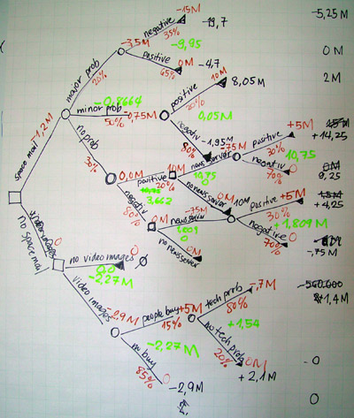
From Wikipedia Manual_decision_tree.jpg.
- In a decision-making process we basically have decisions to make based on evidence
- … and things that might occur randomly
- … and conclusions to reach.
- It is convention to draw these in each in a separate shape of node.
But making business decisions isn't very interesting (to me).
A decision tree can also represent a series of steps taken by an algorithm.
- Each decision is the result of some kind of branch in the algorithm: probably an if/else statement.
- We can look at the various decisions that might be made as part of analyzing the algorithm.
The most common application of this is sorting algorithms.
- We usually counted the running time by looking at the number of decisions made, anyway.
- … since the innermost if/else statement was the thing that ran the most often.
- So, if we can learn something about these trees that sort a list, we'll learn something about all possible (comparison-based) sorting algorithms.
Suppose we're sorting three items (\(a,b,c\)) by comparing them.
- We might start by comparing \(a\) and \(b\).
- If we find out that \(a<b\), then we might move some elements around in the list and then check how \(b\) and \(c\) compare.
- … and so on until we have learned enough to put things in order.
- Our decision tree might look like this:
There are other decision trees for sorting three elements: the details of the algorithm will decide what it looks like.
- We might end up comparing the same elements more than once.
- Or, compare elements unnecessarily (e.g. we learn that \(a<b\) and \(b<c\) but then compare \(a\) and \(c\).)
- But, we accept these things so we get an easy-to-write algorithm.
The worst-case running time of the algorithm is the height of the tree.
If the sorting algorithm is correct, it must have at least \(n!\) leaves.
- … since there are \(n!\) possible orderings of the elements.
So, what kind of binary trees contain \(n!\) leaves?
- Its height must be at least \(\lceil\log_2 n!\rceil\).
- \(\lceil\log_2 n!\rceil\) is \(\Theta(n\log n)\).
- Every comparison-based sorting algorithm has worst-case running time \(\Omega(n\log n)\).
We have a comparison-based sorting algorithm that has worst-case running time \(\Theta(n\log n)\): Mergesort.
- So any other sorting algorithm we find will only be better in constant factor, not growth rate.
Why “comparison-based” sorting?
- Can we sort without comparisons?
- In general, no: \(\Theta(n\log n)\) is the best we can do.
- But if we restrict our input somehow, we can manage. (e.g. we only have integers 1–10.)
- See radix sort, counting sort, bucket sort.