What Every CMPT 225 Student Should Know About Mathematical Induction
- by Brad Bart, Simon Fraser University
Part 1: Overview of Mathematical Induction
Summary
Mathematical induction is a tool to prove, i.e., to make
arguments about, mathematical structures which are self-similar.
In the simplest case, the structure can be stated using a single parameter ![]() ,
where
,
where ![]() spans the positive integers:
spans the positive integers:
![]() .
.
For example, suppose you are interested in the sum of the first
![]() odd integers. That is,
odd integers. That is, ![]() ,
, ![]() ,
, ![]() ,
,
![]() ,
, ![]() and you discover a pattern:
and you discover a pattern:
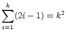
So, you make a guess! ![]() a claim! And you state that the
pattern follows the sequence of integer squares. Written using summation
notation, this claim of yours is
a claim! And you state that the
pattern follows the sequence of integer squares. Written using summation
notation, this claim of yours is
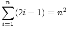 .
And you walk away from the problem, all proud of yourself that you
tried a few instances, found a pattern, and wrote down a closed form.
Basically, you totally pwned it.
.
And you walk away from the problem, all proud of yourself that you
tried a few instances, found a pattern, and wrote down a closed form.
Basically, you totally pwned it.
But then your friend Brad (or at least he says that he's your friend)
asks you how do you know it works for every ![]() .
And you respond that you ``just do'', and that it seemed to fit the
pattern, but Brad just smiles at you, silently. And you realize that
maybe those 4 example cases were probably not enough to ``convince''
someone else, so you show Brad a few more, just for kicks:
.
And you respond that you ``just do'', and that it seemed to fit the
pattern, but Brad just smiles at you, silently. And you realize that
maybe those 4 example cases were probably not enough to ``convince''
someone else, so you show Brad a few more, just for kicks:
He says, ``I see it works for the sums of the first 8 odd numbers, but I
just don't believe it will work for every ![]() .''
.''
Damn your luck! CMPT 225 class is in an hour, which is too little time to verify an infinite number of sample cases. Instead, you put the screws back to Brad.
``OK well, give me an ![]() when it doesn't work!''1
when it doesn't work!''1
And even though Brad can't give you one (probably because he's not that smart) you are still left with the unenviable task of verifying an infinite number of statements before CMPT 225 class starts.
Method of Differences
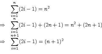
Fortunately, you recall a math trick which you saw in calculus,
known as the method of differences. Since you believe that
your summation is correct, you consider ![]() , and calculate
the value you need to add to it to reach
, and calculate
the value you need to add to it to reach ![]() . That is,
the difference
. That is,
the difference
![]() .
.
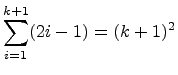
Since the difference is ![]() , which is precisely the
, which is precisely the
![]() term in the summation, you have
proven your closed form holds for incrementally larger
integers
term in the summation, you have
proven your closed form holds for incrementally larger
integers ![]() . And so you go to CMPT 225 class
knowing that you not only pwned the problem, but totally pwned
Brad as well.
. And so you go to CMPT 225 class
knowing that you not only pwned the problem, but totally pwned
Brad as well.
The Inductive Step
What you really did by using the method of differences is a
kind of proof by induction, which, if you recall
the opening paragraph, operates on structures which are
self-similar. In this case, you used the ![]() -term sum
to generate the
-term sum
to generate the ![]() -term sum by adding the
-term sum by adding the
![]() term. Or, algebraically,
term. Or, algebraically,
The technical term for this is the inductive step: to use the verified smaller structures to verify the larger structures. Each of the smaller structures is called an inductive hypothesis.
In a simple induction, like this one, the inductive
step shows that the
![]() case you
verify will imply the
case you
verify will imply the
![]() case.
case.
In a strong induction, the inductive step may use
any combination of verified cases, i.e., the
![]() cases,
in order to imply the
cases,
in order to imply the
![]() case.2
case.2
The Basis Cases
The inductive step is a powerful engine indeed.
For the squares example, the
![]() case
relies on the
case
relies on the
![]() case, so you can
verify any case as high as you like, i.e., for all positive
integers
case, so you can
verify any case as high as you like, i.e., for all positive
integers ![]() . Well, almost all. The inductive step doesn't
verify the
. Well, almost all. The inductive step doesn't
verify the
![]() case, because no
case comes before it!
case, because no
case comes before it!
The
![]() case is a special case called
a basis case. It is special because you must verify it
using another method besides the inductive step.
It turns out that you already did
this when you tested out the first few sums: you verified the
case is a special case called
a basis case. It is special because you must verify it
using another method besides the inductive step.
It turns out that you already did
this when you tested out the first few sums: you verified the
![]() case (as well as the
case (as well as the
![]() ,
,
![]() , and
, and
![]() cases)
when you were searching for your general pattern.
cases)
when you were searching for your general pattern.
For simple induction, you only have to verify one basis case: ![]() .
For strong induction, it may be several cases: whatever your
inductive step doesn't cover.
The process of verifying these cases is known as the basis step.
The combination of the inductive step and basis step
is a proof by induction.3
.
For strong induction, it may be several cases: whatever your
inductive step doesn't cover.
The process of verifying these cases is known as the basis step.
The combination of the inductive step and basis step
is a proof by induction.3
Sidebar: All of you have seen proofs by induction before, most notably in MACM 101. It is important that you are comfortable with the mechanics of a proof by induction before proceeding to Parts 2 and 3. To bone up, there are worked examples and exercises for you to try.
In most of the examples that follow, we will skip the basis step, which is pretty common for usage by computer scientists, like yourself. Why? Because you just aren't likely to assert a claim without first verifying a few small cases!
But please note that the basis step is treasured by some overly
skeptical mathematicians who know that the inductive step on
its own is not strong enough as a general proof.
This is because it is possible to
prove the inductive step on something that is always false.
For example, the method of differences works on
 .
The mathematicians aren't wrong about this, but then again
they aren't as practical as yourself.
.
The mathematicians aren't wrong about this, but then again
they aren't as practical as yourself.
Now just because you aren't going to prove any basis cases doesn't mean you should just forget about them either. They have a strong relation to the base cases of recursive algorithms.
How Induction Relates to Computer Science
Induction and Recursion
Recursion is an algorithmic technique where you solve a problem by using the solutions to smaller instances of the same problem.
The inductive step from the squares example was recursive because
in order to verify the
![]() case, you relied
on the
case, you relied
on the
![]() case. But similarly,
case
case. But similarly,
case ![]() depended on case
depended on case ![]() . And case
. And case ![]() depended on case
depended on case ![]() ,
which depended on case
,
which depended on case ![]() ,
, ![]() , which depended on case 3, which
depended on case 2, which depended on case 1. And since case 1 was
verified in the basis step, you concluded the
, which depended on case 3, which
depended on case 2, which depended on case 1. And since case 1 was
verified in the basis step, you concluded the
![]() case was true.
case was true.
This sort of recursive reasoning, where you break down the large case
into smaller cases, is known as the top-down approach.
In this example, it leads directly to a recursive implementation of the
function SumOdd(n), which for positive n returns the
sum of the first n odd integers: the resulting sum
is based on a call to SumOdd(n-1), when n ![]() .
The case for
.
The case for n ![]() , where the recursion stops, is the
base case.
, where the recursion stops, is the
base case.
int SumOdd(int n) {
  // base case
  if (n == 1) return 1;

  // recursive case
  return SumOdd(n-1) + (2*n - 1);
}
Induction and Iteration
The other way to look at induction is by starting with case 1, the basis case. Then, by using the inductive step, case 1 implies case 2. Now that you have case 2, you use the inductive step again, and you have case 3. Case 3 implies case 4, which implies case 5, which implies case 6, and so on, climbing your infinite ladder, rung by rung, going as high as you like.
This sort of recursive reasoning, where you use the smaller cases to
build up to the large case, is known as the bottom-up approach.
In the squares example, it leads directly to an iterative implementation
of the function SumOdd(n), defined as before. This time a
running total holds the sum of the first i-1 odd integers.
In each iteration, the i
![]() odd integer
is added to the running sum.
odd integer
is added to the running sum.
int SumOdd(int n) {
  total = 1;
  for (int i = 2; i <= n; ++i) {
    // assert(total == (i-1)*(i-1));
    total += (2*i - 1);
    // assert(total == i*i);
  }
}
The two assertions in the implementation serve to convince the
reader that the code does just what it is supposed to do: that at
the beginning of the loop
Loop Invariants
The loop invariants for SumOdd(n) look very much like the
inductive step. This is not a coincidence. Loop invariants are
usually statements about an algorithm that you can prove by
induction. The most useful invariants will be about either:
As an example, consider the algorithm Insertion Sort on the
integer array A[0..n-1]:
void isort(int *A, int n) {
  for (int i = 1; i < n; i++) {
    // insert A[i] into A[0..i-1]
    int temp = A[i];
    int j = i-1;

    // shift all A[] > temp
    while (j >= 0 && A[j] > temp) {
      A[j+1] = A[j];
      j--;
    }
    A[j+1] = temp;
  }
}
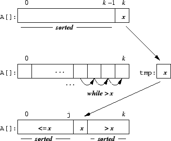
To explain the algorithm, the correct position of A[i] is
located by finding all those elements to its left which are larger.
Those elements are shifted up by one position to make
space for the insertion of A[i]. A demonstration on
an array of 7 elements:
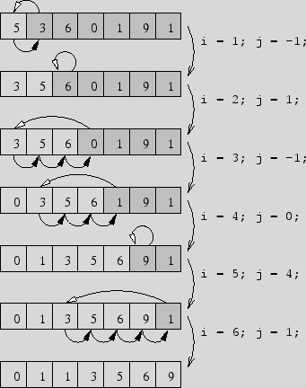
Insertion Sort is an incremental sort.
Each loop begins with a sorted A[0..i-1], and the
element A[i] is joined to it such that the
result is a sorted A[0..i]. In other words:
At the beginning of each loop,This is a loop invariant about the progress of the algorithm.A[0..i-1]is a sorted permutation of the firstielements ofA[], and at the end of each loopA[0..i]is a sorted permutation of the firsti+1elements ofA[].
Once you have declared a loop invariant, your next goal is to prove it by induction. Why? Because the byproduct of your proof will be a proof of correctness of the algorithm.
Remember that the goal of a sorting algorithm is to permute
the elements of A[0..n-1] such that they are in
sorted order. At the end of the final loop, i.e., when
i = n-1, the result will be a sorted permutation
of the first n elements of A[].
Proof (by induction on i):
Inductive Step: Assume all loop invariants hold for
all loop indices i ![]() , and conclude that they hold
for the loop index
, and conclude that they hold
for the loop index i ![]() .
.
Certainly, A[0..k-1] is sorted at the beginning of the
loop i ![]() , because it was sorted at the end of loop
, because it was sorted at the end of loop
i ![]() .
.
To show that
A[0..k] is sorted at the end of the loop
i ![]() , we follow the execution of the loop body.
Let
, we follow the execution of the loop body.
Let ![]()
A[k].
Informally speaking, the while loop shifts elements to a
higher index, as long as they are greater than ![]() . Since that
portion of the list was sorted, it remains sorted, because the
order is maintained on an incremental shift.4 When the loop terminates,
the value of
. Since that
portion of the list was sorted, it remains sorted, because the
order is maintained on an incremental shift.4 When the loop terminates,
the value of j is such that A[0..j] ![]()
A[j+2..k]. The final step of assigning
A[j+1]
![]() generates a sorted
generates a sorted A[0..k]. ![]()
And now to declare an invariant about the running time. Because the inner while loop runs an indefinite number of times, it will be impossible to construct an invariant that states the running time as an equation. Instead, the loop invariant will be a description of the worst case, i.e., the largest number of steps, using an inequality.
On each iteration of the while loop, there are
2 comparisons for testing the entry condition and
2 assignment operations for shifting A[j] and
updating j. In the worst case, this will run
until j = -1, costing one more comparison.
Therefore, the total running time of the inner loop must be
![]() i
i![]() operations.
operations.
Each iteration of the outer for loop performs
3 assignment operations plus at most
![]() i
i![]() operations for the inner
while, so the running time of the
operations for the inner
while, so the running time of the
i
![]() outer loop must be
outer loop must be
![]() i
i![]() operations.
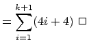
Therefore, the loop invariant for the running time
of insertion sort is:
operations.
Therefore, the loop invariant for the running time
of insertion sort is:
The total running time,, of the loops i
, satisfies:
Proof (by induction on.
Since ![]() , the total running time to run
loops i
, the total running time to run
loops i
![]() ,
equals the sum of
,
equals the sum of ![]() , the total running time to run
loops i
, the total running time to run
loops i
![]() , plus the time to
run the loop i
, plus the time to
run the loop i ![]() , we have
, we have
![$\displaystyle \leq \displaystyle{\sum_{i=1}^{k} (4i+4)} + [4(k+1)+4]$](img66.png) |
||
 |
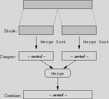
Invariants and Recursive Algorithms
Recursive Algorithms often solve problems using the Divide & Conquer paradigm, which involves three stages: divide, conquer and combine.
// sorts A[first..last]
void msort(int *A, int first, int last) {
  // base case
  if (first >= last) return;

  // divide
  int mid = (first+last) / 2;

  // conquer
  msort(A, first, mid);
  msort(A, mid+1, last);

  // combine
  merge(A, first, mid, last);
}
Just like an inductive step for a strong induction,
it is assumed that the algorithm is correct for all
smaller cases, and therefore the conquer stage
correctly sorts the two sublists A[first..mid] and
A[mid+1..last]. The merge(...) step
results in a sorted A[first..last].
This analysis illustrates how powerful invariants are for
proving recursive algorithms correct.
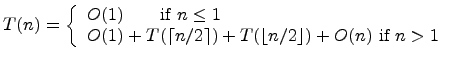
The analysis of the running time is similar.
Let ![]() represent the number of steps to Merge Sort
an
represent the number of steps to Merge Sort
an ![]() element array. When
element array. When ![]() , the array
, the array A
is trivially sorted (base case), and the running time
is ![]() . When
. When ![]() , a certain number of steps are
taken for each of the Divide, Conquer and
Combine stages.
, a certain number of steps are
taken for each of the Divide, Conquer and
Combine stages.
mid costs
The next step is a familiar one: guess an expression for ![]() and then use induction to prove it is correct. Because you
remember past discussions of the running times of sorting
algorithms, you guess that
and then use induction to prove it is correct. Because you
remember past discussions of the running times of sorting
algorithms, you guess that
![]() , i.e.,
for constants
, i.e.,
for constants ![]() , the inequality
, the inequality
![]() holds for every
holds for every
![]() .
.
The inductive proof is beyond the scope of CMPT 225, but you will do proofs like this in CMPT 307. If you are keen to see this analysis to its proper conclusion, click here.
Induction and Recursion in CMPT 225
Induction, Recursion and Elementary Data Structures
In your intro computing classes, there were only two known
data structures: the array and the linked list,
and you did an implementation of a dynamic set using each.
Since both provided a linear data layout, then at least one
of the two operations, insert and search, took
![]() time where
time where ![]() represents the current size of the set.
represents the current size of the set.
Both arrays and linked lists are recursive in that you can build a larger one out of an incrementally smaller one plus an extra element. This means you can prove the correctness and the running time of algorithms on these data structures, by using simple induction, much like you did for Insertion Sort.
figure
Similarly, within an array are many smaller subarrays, not just incrementally smaller. The same can be said for all of the sublists of a linked list. This means you can prove the correctness and the running time of algorithms on these data structures, by using strong induction, much like you did for Merge Sort.
figure
Case Study: Dynamic Set Implementation Using an Array
To build a dynamic set using a data structure requires you to
think about how to lay out the data in your structure. In the
case of an array, it is probably easiest to insert into the
first free slot of the array, which is an ![]() operation.
operation.
void insert(int key) {
  A[len++] = key;
}
The keys are placed at the array indices in the order in which
they were inserted, thus they may not appear in sorted order.
Therefore, to search the set for a key, a linear search is required.
// linear search - returns -1 if not present
int search(int key) {
  for (int i = 0; i < len; i++)
    if (key == A[i]) return i;
  return -1;
}
But instead if the collection is a sorted array then the
search operation can run in
The resulting recursive relation,
![]() ,
...
Binary search runs in
,
...
Binary search runs in
![]() steps, which is
steps, which is
// binary search - returns -1 if not present
int search(int key) {
  int first = 0, last = len-1;
  while (first < last) {
    int mid = (first+last)/2;
    if (A[mid] < key) // search upper half
      first = mid + 1;
    else // search lower half
      last = mid;
  }
  if (A[first] == key) return first;
  else return -1;
}
void insert(int key) {
  // shift all A[] > key
  int j = len-1;
  while (j >= 0 && A[j] > key) {
    A[j+1] = A[j];
    j--;
  }
  A[j+1] = key;
  len++;
More Complex Linked Data Structures
The implementation of a dynamic set using a sorted array yielded an excellent running time for search at the expense of insert. Ideally, you should seek an implementation that has an excellent running time for both operations.
Strategy: Divide & Conquer!
Like for binary search, arrange elements so that the query of 1 element eliminates roughly half of the set. In this case, use a more complex linked data structure: a binary tree. A binary tree is a (possibly empty) rooted tree, where each node has at most two children, denoted left and right. Each node in the tree contains a key, where the keys are related by the following property:
figure
Recursive definition of binary search tree (BST)
- a dynamic set is implemented as a (possibly empty) binary tree
- subtrees ![]() ,
, ![]() are dynamic sets
-
are dynamic sets
-
![]()
So, to search for a key or insert a new key, traverse down the
tree examining each key ![]() as you go. If key
as you go. If key ![]() , then you
recurse left, if key
, then you
recurse left, if key ![]() , then you recurse right, just like
for binary search. The running time for each operation is
, then you recurse right, just like
for binary search. The running time for each operation is
![]() , where
, where ![]() is the height of the binary tree. When the
tree is roughly balanced,
is the height of the binary tree. When the
tree is roughly balanced,
![]() .
.
figure
Priority Queue Implementations
A priority queue is like a regular queue in that it is a collection of keys which you insert and remove. But in this version, each key has a priority number associated with it: the lower the number, the higher the priority. So, the next key to remove is the one with the highest priority.
Case Study: Priority Queue Implementation Using an Array
Using a reverse sorted array gives an ![]() insert and an
insert and an
![]() remove. You should implement this as an exercise
to convince yourself.
remove. You should implement this as an exercise
to convince yourself.
Just like for the dynamic set implementation using an array,
insert into the first unoccupied slot: running time ![]() .
To remove the minimum requires a linear search for the smallest,
swapped with the last occupied slot: running time
.
To remove the minimum requires a linear search for the smallest,
swapped with the last occupied slot: running time ![]() .
.
void insert(int key, int priority) {
    A[len++] = Node(key, priority);
}
int remove() {
  int smallest = A[0].priority;
  int smallestpos = 0;
  for (int pos = 1; pos < len; pos++)
    if (A[pos].priority < smallest.priority) {
      smallest = A[pos].priority;
      smallestpos = pos;
    }
  int ret = A[pos].key;
  A[pos] = A[--len];
  return ret;
}
and an if you used either as a container
After Beyond trees
The loop invariant for the running
Therefore, its cost is The outer for loop runs n - 1 times, but
Consider the
i
![]() loop
loop
![]() case. But similarly,
To verify the
case. But similarly,
To verify the
![]() case, you relied
case, you relied
Since recursion operates on structures which are self-similar, it behaves
Do you remember what I wrote at the beginning?
``Mathematical induction is a tool to prove mathematical structures which are self-similar.''
Here, you used a smaller case (the
![]() case)
to prove a larger one (the
case)
to prove a larger one (the
![]() case).
And that's what self-similar means, that the smaller
structures can be used to prove the larger ones.
case).
And that's what self-similar means, that the smaller
structures can be used to prove the larger ones.
The Inductive Step
To make the notation more compact, you define the predicate
![]() : the sum of the first
: the sum of the first ![]() odd integers equals
odd integers equals ![]() ,
or more compactly:
,
or more compactly:
.
To make quick work of verifying your infinite number of statements,
you show that for any ![]() , if you knew it was true for the
case where
, if you knew it was true for the
case where ![]() , then you can use that fact to show it's true
for
, then you can use that fact to show it's true
for ![]() . In other words,
. In other words, ![]() implies
implies ![]() .
.
This implication is called the inductive step.
Because the statements are self-similar, you can If you can show that
![]() sum
sum
inductive hypothesis
basis case
bottom up vs top down
analogies
strong induction
examples
- sums
- divisibility
- gcd
- demoivre's theorem
- trees
- geometry: tiling
exercises
- write a computer program that takes as input integers ![]() such that
such that
![]() and
and
![]() and outputs a
and outputs a
![]() grid, completely tiled by trominos, except for
the grid square
grid, completely tiled by trominos, except for
the grid square ![]() .
solutions
.
solutions
Connections with Computer Science
We can do this because summations are self-similar, that is, they . summation: total = 0; for (int i = 0; i < N; i++) total += A[i]; invariants recursion trees
Appendix: Writing Proofs By Induction
This section supplies a systematic approach to completing
proofs by induction. In all parts included here, you may
assume the statement to be proven is the predicate ![]() ,
for all integers
,
for all integers ![]() .
.
The Framework
A proof by induction involves two main steps: the inductive step and the basis step. The inductive step is the harder (and more important) work of the two. What is involved on each step depends on what sort of induction you are facing:
Your goal for the basis step is to verify ![]() .
.
Your work in the basis step is to verify those cases which cannot be concluded by the inductive step. Usually it will be 2 or more cases.
Strategy for Proving The Inductive Step
The inductive step is the most important part of a proof by induction. The rest are just details. And here's the key:
You must use the inductive hypothesis, ![]() , to prove
, to prove ![]() .
.
Because the statements are self-similar, you should be able to find
![]() ``within''
``within'' ![]() . Usually, it takes a few steps, but by
factoring, splicing, or by doing algebra, you can rearrange
. Usually, it takes a few steps, but by
factoring, splicing, or by doing algebra, you can rearrange ![]() to make it look like
to make it look like ![]() .
.
Examples
1. Summations
Prove that
for all
![]() .
.
Strategy: Proofs by induction on summations are friendly, because within any sum, there is always an incrementally smaller sum. This is the self-similarity you can exploit in the inductive step.
Proof (by induction on ![]() ):
):
Let ![]() :
.
:
.
Inductive Step: Assume ![]() is true for some arbitrary
is true for some arbitrary ![]() ,
i.e., that
,
i.e., that
 .
The goal is to conclude
.
The goal is to conclude ![]() ,
i.e., that
,
i.e., that
 .
.
Strategy: You could prove
![]() by adding
by adding ![]() to both sides of
the Inductive Hypothesis, which is the same approach you took when you used
the method of differences to prove this earlier. But in proofs by induction,
it is more common to find a substitution for
to both sides of
the Inductive Hypothesis, which is the same approach you took when you used
the method of differences to prove this earlier. But in proofs by induction,
it is more common to find a substitution for ![]() , so that's what
you'll do here. To make
the substitution easier to see, cleave the
, so that's what
you'll do here. To make
the substitution easier to see, cleave the
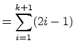
![]() term in the summation.
term in the summation.
Verify the inductive step by showing the left-hand-side equals the right-hand-side:
 |
||
![$\displaystyle = \displaystyle{\sum_{i=1}^{k}} (2i-1) + [2(k+1) - 1]$](img120.png) |
||
| (Recursive Definition of |
||
| |
||
Basis Step: Verify ![]() for
for ![]() .
.
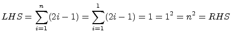 .
.
Since the inductive step and basis step have been proven, then
by the Principle of Mathematical Induction, ![]() is proven
for all integers
is proven
for all integers ![]() .
. ![]()
2. Divisibility
Prove that
![]() is evenly divisible by 8 for all
is evenly divisible by 8 for all ![]() .
.
Strategy: As usual, the goal is to find the inductive
hypothesis within ![]() . But this case is a little
different because there are no equations.
. But this case is a little
different because there are no equations.
Proof (by induction on ![]() ):
):
Let ![]() :
:
![]() is evenly divisible by 8.
is evenly divisible by 8.
Inductive Step: Assume ![]() is true for some arbitrary
is true for some arbitrary ![]() ,
i.e., that
,
i.e., that
![]() is evenly divisible by 8.
The goal is to conclude
is evenly divisible by 8.
The goal is to conclude ![]() ,
i.e., that
,
i.e., that
![]() is evenly divisible by 8.
is evenly divisible by 8.
Strategy: Unlike for the summation, where a simple
operation (i.e., adding one term) transformed ![]() into
into ![]() ,
the strategy for this proof is not so clear. There is an algebraic
trick that almost always works: add and subtract terms to construct a
copy of the inductive hypothesis.
,
the strategy for this proof is not so clear. There is an algebraic
trick that almost always works: add and subtract terms to construct a
copy of the inductive hypothesis.
Basis Step: Verify ![]() for
for ![]() .
.
![]() , which is clearly divisible by 8.
, which is clearly divisible by 8.
And by the Principle of Mathematical Induction, ![]() is true
for all integers
is true
for all integers ![]() .
. ![]()
3. Inequalities
Prove that
![]() , for real
, for real ![]() and
integer
and
integer ![]() .
.
Proof: When ![]() ,
,
![]() and
and
![]() ,
so they are equal.
,
so they are equal.
Inductive Step:
Given that
![]() , for some arbitrary
, for some arbitrary ![]() (Inductive Hypothesis),
show that
(Inductive Hypothesis),
show that
![]() .
.
By the Principle of Mathematical Induction, the result follows.
![]()
![]() leads to
leads to ![]()
Proof: Let ![]() be the statement shown above.
We intend to prove
be the statement shown above.
We intend to prove ![]() true for all
true for all ![]() .
This is the best we can do because
.
This is the best we can do because ![]() is false for
is false for ![]() .
.
![]()
Suppose ![]() is true for an arbitrarily chosen
is true for an arbitrarily chosen ![]() , i.e.,
, i.e.,
![]() .
.
Show ![]() is true, i.e.,
is true, i.e.,
![]() .
.
By the Principle of Mathematical Induction, the result follows.
4. Geometry
Tiling with trominos.
5. Sequences
Fibonacci proofs.
Fibonacci ![]()
6. Sets?
Exercises
Pell's equation:
![]() ?
?